Market prices generally respond to an increase in supply or demand. This phenomenon, called “price impact,” is of central importance in financial markets. Price impact provides feedback between supply and demand, an essential component of the price discovery mechanism. Price impact also accounts for the vast majority of large traders’ execution costs — costs which regulators may seek to reduce by tweaking market structure.

Price impact is a concave function of meta-order [1] size — approximately proportional to the square-root of meta-order size — across every well-measured financial market (e.g. European and U.S. equities, futures, and bitcoin). There are some nice models that help explain this universality, most of which require fine-grained assumptions about market dynamics. [2] But perhaps various financial markets, regardless of their idiosyncrasies, share emergent properties that could explain empirical impact data. In this post, I try to predict price impact using only conjectures about a market’s large-scale statistical properties. In particular, we can translate intuitive market principles into integral equations. Some principles, based on efficiency arguments, imply systems of equations that behave like real markets.

In part I, we’ll start with the simplest principles, which we’ll only assume to hold on average: the “fair pricing condition”, and that market prices efficiently anticipate the total quantity of a meta-order based on its quantity already-executed. In part II, we’ll replace the fair pricing condition with an assumption that traders use price targets successfully, on average. In part III, we’ll return to fair pricing, but remove some efficiency from meta-order anticipation — by assuming that execution information percolates slowly into the marketplace. In part IV, we’ll emulate front-running, by doing the opposite of part III: leaking meta-orders’ short-term execution plans into the market. In parts V and VI, we’ll discuss adding the notion of urgency into meta-orders.

Definitions and Information-Driven Impact

We can motivate price impact from a supply and demand perspective. During the execution of a large buyer’s meta-order, her order flow usually changes the balance between supply and demand, inducing prices to rise by an amount called the “temporary price impact.” After the buyer is finished, she keeps her newly-acquired assets off the market, until she decides to sell. This semi-permanent reduction in supply causes the price to settle at a new level, which is higher than the asset’s initial price by an amount called the “permanent price impact.” Changes in available inventory cause permanent impact, and changes in flow (as well as inventory) cause temporary impact. [3]

Another view is that informed trading causes permanent impact, and that uncertainty about informedness causes temporary impact. When a trader submits a meta-order, its permanent impact should correspond in some fashion to her information. And its temporary impact should correspond to the market-estimate of permanent impact. In an “efficient” market, the informational view and the supply/demand view should be equivalent.

Before we proceed, we need some more definitions. Define $\alpha(q)$ as the typical permanent price impact associated with a meta-order of quantity $q$ . By “typical”, I mean that $\alpha(q)$ is the expectation value of permanent impacts, $\alpha_{s}(q)$ , associated with a situation, $s$ , in the set of all possible situations and meta-orders, $S$ . Specifically, $\alpha(q) = \mathbf{E}_{s \in S}[\alpha_{s}(q)]$ . It’s reasonable to associate the colloquial term “alpha” — which describes how well a given trade ( $s$ ) predicts the price — with $\alpha_{s}$ .

Also define $\mathcal{I}(q)$ as the typical temporary price impact after a quantity $q$ has been executed. Again, “typical” means $\mathcal{I}(q) = \mathbf{E}_{s \in S}[\mathcal{I}_{s}(q)]$ .

These expectations can be passed through the integrals discussed below, so we don’t need to pay attention to them. In the rest of this post, “permanent impact” will refer to the expectation $\alpha(q)=E_{s \in S}[\alpha_{s}(q)]$ unless otherwise specified (and likewise for “temporary impact” and $\mathcal{I}(q)$ ).

I. A Bare-Bones Model

Starting from two assumptions of market efficiency, we can determine the typical price-trajectory of meta-orders. The two conditions are:

I.1) The “fair pricing condition,” which equates traders’ alpha with their execution costs from market-impact (on average):

$\alpha(q) = \frac{1}{q} \int_{0}^{q} \mathcal{I}(q') dq'$

The integral denotes the quantity-averaged temporary impact “paid” over the course of an entire meta-order. “Fair pricing” means that, in aggregate, meta-orders of a given size do not earn excess returns or below-benchmark returns.

Temporary price impact (black line) over the course of a meta-order of size $q$ . After the execution is finished, the price impact decays (dashed line) to $\alpha(q)$ (red), the quantity-weighted average of the meta-order’s temporary impact trajectory

I.2) Efficient linkage between temporary and permanent price impact:

$\mathcal{I}(q') = \mathbf{E}_{q}[\alpha(q)|q \geq q'] = \int_{q'}^{\infty} \alpha(q)p[q|q \geq q']dq$

Here, $p[q]$ is the PDF of meta-order sizes and $P[q]$ is the CDF. And $p[q|q \geq q']$ is the truncated probability density of meta-order sizes, $\frac{p[q]}{1 - P[q']}$ — which represents the probability distribution of $q$ given that quantity $q'$ from the meta-order has already executed. This condition means that, on average, “the market” observes how much quantity an anonymous trader has executed, and uses that to estimate the distribution of her meta-order’s total quantity. “The market” then calculates an expectation value of the meta-order’s alpha, which sets the current clearing price (i.e. temporary impact). [4] [5] To emphasize, only the average temporary impact is determined this way; a single meta-order could have much different behavior. Here’s a heuristic example:

A. A trader is buying a lot of IBM stock and has so far bought a million shares.
B. The rest of the market sees signs (like higher price and volume) of that purchase and knows roughly that somebody has bought a million shares.
C. Once a trader has bought a million shares, there is a 50% chance that she’ll buy 5 million in total, and a 50% chance that she’ll buy 10 million. “The market” knows these probabilities.
D. For 5 million share meta-orders, the typical permanent price impact is 1%, and for 10 million share meta-orders it’s 2%. So “the market” expects our trader’s meta-order to have permanent impact of 1.5%. The typical temporary impact is determined by this expectation value. This particular meta-order may have temporary impact smaller or larger than 1.5%, but meta-orders sent under similar circumstances will have temporary impact of 1.5% on average.

An illustration of this linkage. The temporary price impact trajectory is the black line. At a given value of $q'$ , $\mathcal{I}(q')$ (blue) is equal to the expected value (blue) of the permanent price impact given that the meta-order has size $q'$ or bigger. The probability density of the final meta-order size, $p[q|q \geq q']$ , is shown in shaded red. The permanent impact associated with those meta-order sizes is shown in green.

Relationship with Efficiency

The fair pricing condition could emerge when the capital management industry is sufficiently competitive. If a money manager uses a trading strategy that’s profitable after impact costs, other managers could copy it and make money. The strategy would continue to attract additional capital, until impact expenses balanced its alpha. (Some managers are protective of their methods, but most strategies probably get replicated eventually.) If a strategy ever became overused, and impact expenses overwhelmed its alpha, then managers would probably scale back or see clients pull their money due to poor performance. Of course these processes take time, so some strategies will earn excess returns post-impact and some strategies may underperform — fair pricing would hold so long as they average out to a wash.

A strictly stronger condition than I.2) should hold in a market where meta-orders are assigned an anonymous ID, and every trade is instantly reported to the public with its meta-order IDs disclosed. Farmer, Gerig, Lillo, and Waelbroeck call a similar market structure the “colored print” model. Under this disclosure regime, if intermediary profits are zero, the expected alpha would determine the temporary impact path of individual meta-orders, not just the average $\mathcal{I}(q')$ as in I.2). All meta-orders would have the same impact path: $\mathcal{I}_{s}(q') = \mathbf{E}_{q}[\alpha(q)|q \geq q'] = \int_{q'}^{\infty} \alpha(q)p[q|q \geq q']dq$ for any $s$ . [6] Now, the colored print model doesn’t seem very realistic; most markets don’t have anywhere near that level of transparency. Nonetheless, Farmer et al. show preliminary measurements that partly support it. [7]

Even without colored prints, the linkage property I.2) could be due to momentum and mean-reversion traders competing away their profits. As discussed by Bouchaud, Farmer, and Lillo, most price movement is probably caused by changes in supply and demand. That is, if prices move on increased volume, it’s likely that someone activated a large meta-order, especially if there hasn’t been any news. So, if average impact overshot I.2) significantly, a mean-reversion trader could plausibly watch for these signs and profitably trade opposite large meta-orders. Likewise, if average impact undershot I.2), momentum traders might profit by following the price trend.

Solving the System of Equations

We can combine I.1) and I.2) to get an ODE [8]:

$\alpha''(q) + (\frac{2}{q} - \frac{p[q]}{1-P[q]})\alpha'(q) = 0$

This ODE lets us compute $\alpha(q)$ and $\mathcal{I}(q)$ for a given meta-order size distribution, $p[q]$ .

It’s common to approximate $p[q]$ as a $Pareto[q_{min},\beta]$ distribution ( $p[q] = \frac{\beta q_{min}^{\beta}}{q^{\beta+1}}$ ). If we do so, then $\frac{p[q]}{1-P[q]} = \frac{\beta}{q}$ , and the ODE has solution $\alpha(q) = c_1 q^{\beta-1}+c_2$ . Equation I.1) implies $\mathcal{I}(q) = \alpha(q)+q\alpha'(q)$ , so we have that $\mathcal{I}(q) = c_1 \beta q^{\beta-1} + c_2$ . Impact should nearly vanish for small $q$ , so we can say that $c_2 \approx 0$ . The post-execution decay in impact is then given by $\frac{\alpha(q)}{\mathcal{I}(q)} = \frac{1}{\beta}$

If we choose $\beta = \frac{3}{2}$ (roughly in-line with empirical data), we get the familiar square-root law: $\mathcal{I}(q) \propto \sqrt{q}$ . We also get an impact ratio of $\frac{\alpha(q)}{\mathcal{I}(q)} = \frac{2}{3}$ , very close to real-world values.

A similar method from Farmer, Gerig, Lillo, and Waelbroeck gives the same result. They use the fair pricing condition, but combine it with a competitive model of market microstructure. [9] Here, instead of having a specific model of a market, we’re making a broad assumption about efficiency with property I.2). There may be a large class of competitive market structures that have this efficiency property.

Distribution of Order Sizes Implied by a Given Impact Curve

Under this model, knowing an asset’s price elasticity ( $\mathcal{I}(q)$ ) is equivalent to knowing its equilibrium meta-order size distribution( $p[q]$ ). [10] If a market impact function $\mathcal{I}(q)$ is assumed, we can calculate the meta-order size distribution. [11] For instance, Zarinelli, Treccani, Farmer, and Lillo are able to better fit their dataset with an impact function of the form $\mathcal{I}(q) = a Log_{10}(1+bq)$ (p17). This impact curve implies a $p[q]$ that’s similar to a power-law, but with a slight bend such that its tail decays slower than its bulk:

Meta-order size distribution implied by the impact curve $\mathcal{I}(q) = 0.03 Log_{10}(1+470q)$ , which Zarinelli, Treccani, Farmer, and Lillo fit to their dataset of single-day meta-orders. In this case, $q$ would be analogous to their chosen measure of size, the daily volume fraction $\eta$ . The impact function’s fit might be invalid for very large meta-orders ( $q \approx 1$ ), so the lack of a sharp cutoff near $q \approx 1$ in the implied size distribution isn’t problematic.

II. A Replacement Principle for Fair Pricing: Traders’ Effective Use of Price Targets

The two integral equations in part I can be modified to accommodate other market structure principles. There’s some evidence that our markets obey the fair pricing condition, but it’s fun to consider alternatives. One possibility is that traders have price targets, and cease execution of their meta-orders when prices approach those targets. We can try replacing the fair pricing of I.1) with something that embodies this intuition:

II.1) $\alpha(q) = a\mathcal{I}(q) + d$

Where $a$ and $d$ are constants. This principle should be true when traders follow price-target rules, and their targets accurately predict the long-term price (on average). If $d=0$ and $a=\frac{5}{4}$ , then traders typically stop executing when the price has moved $\frac{4}{5}$ of the way from its starting value to its long-term value. If $a=1$ and $d=0.01$ , then traders stop executing when the price is within 1% of its long-term value.

If we keep I.2), this gives the ODE:

$\alpha'(q) + \frac{p[q](a-1)}{1 - P[q]}\alpha(q) + \frac{p[q]d}{1 - P[q]}=0$

It’s readily solved. [12] In particular, if $q \sim Pareto[q_{min},\beta]$ and $a \neq 1$ :

$\alpha(q) = c q^{\beta (1-a)}+\frac{d}{1-a}$ and $\mathcal{I}(q) = \frac{c q^{\beta (1-a)}+\frac{d}{1-a}-d}{a}$ .

For typical values of $\beta \approx 1.5$ , we can get the usual square root-law by setting $a \approx \frac{2}{3}$ . We need $0 < a < 1$ in order for impact to be a concave, increasing function of order size, in agreement with empirical data. This suggests that perhaps traders do employ price targets, only instead of being conservative, their targets are overly aggressive. In other words, this model gives a realistic concave impact function if traders are overconfident and think their information is worth more than it is. [13] More generally, the partial reversion of impact after meta-orders’ completion could be explained with overconfidence. And when the “average” trader is overconfident just enough to balance out her alpha, the market will obey the fair pricing condition. I think there’s more to fair pricing than overconfidence, but this link between human irrationality and market efficiency is intriguing.

III. A Replacement Principle for Efficient Linkage, with Delayed Dissemination of Information

We can also think about alternatives for I.2). In I.2), “the market” could immediately observe the already-executed quantity of a typical meta-order. But markets don’t instantly process new information, so perhaps the market estimate of meta-orders’ already-executed quantity is delayed:

III.2) $\mathcal{I}\left(q'\right) = \mathbf{E}_{q}[\alpha(q)|q \geq (q'-q_d)^+] = \frac{\int_{(q'-q_d)^+}^{\infty } p[q] \alpha (q) \, dq}{1-P[(q'-q_d)^+]}$

Where $q_d$ is a constant and $(q'-q_d)^+$ is the positive part of $(q'-q_d)$ : $max(0,(q'-q_d))$ .

This condition should be true when the market (on average) is able to observe how much quantity an anonymous trader executed in the past, when her executed quantity was $q_d$ less than it is in the present. This information can be used to estimate the distribution of her meta-order’s total size, and thus an expectation value of its final alpha. The temporary impact is set by this expectation value.

Intuitively, small meta-orders may blend in with background activity, but large ones are too conspicuous. If someone sends two 100-share orders to buy AAPL, other traders won’t know (or care) whether those orders came from one trader or two. But if a large buyer is responsible for a third of the day’s volume, other traders will notice and have a decent estimate of the buyer’s already-executed quantity, even if they don’t know whether the buyer was involved in the most recent trades on the tape. So, it’s very plausible for market participants to have a quantity-lagged, anonymized view of each other’s trading activity.

Combining III.2) with fair pricing I.1) gives the delay differential equation [14]:

$\begin{cases} q \alpha ''(q) + \alpha '(q) \left(2-\frac{q p[q-q_d]}{1-P[q-q_d]}\right)-\left(\alpha (q)-\alpha (q-q_d)\right)\frac{p[q-q_d]}{1-P[q-q_d]}=0, & \mbox{if } q \geq q_d \\ \mathcal{I}(q)=\alpha(q)=constant, & \mbox{if } q < q_d \end{cases}$ .

We can solve it numerically [15]:

$\mathcal{I}(q)$ and $\alpha(q)$ when $q$ is Pareto-distributed, for several values of $q_d$ . The general behavior for $q \gg q_d$ is similar to that of $q_d=0$ , as in I.

The impact ratio $\frac{\alpha(q)}{\mathcal{I}(q)}$ for several values of $q_d$ . This ratio is 1 when the price does not revert at all post-execution, and 0 when the price completely reverts.

I gather that fundamental traders don’t like it when the price reverts on them, so some may want this impact ratio to be close to 1. Delayed information dissemination helps accomplish this goal when meta-orders are smaller than what can be executed within the delay period. But traders experience bigger than usual reversions if their meta-orders are larger than $q_d$ . This behavior is intuitive: if a meta-order has executed a quantity less than $q_d$ , other traders will have zero information about it and can’t react. But as soon as its executed quantity reaches $q_d$ , the market is made aware that somebody is working an unusually big meta-order, and so the price moves considerably.

Some bond traders are pushing for a longer delay in trade reporting. One rationale is that asset managers could execute meta-orders during the delay period, before other traders react and move the market. The idea feels superficially like condition III.2), but isn’t a perfect analogy, because counterparties still receive trade confirmations without delay. And counterparties do use this information to trade. [16] So, delaying prints may not significantly slow the percolation of traders’ information into the marketplace, it just concentrates that information into the hands of their counterparties. Counterparties might provide tighter quotes because of this informational advantage, but only if liquidity provision is sufficiently competitive. [17]

In theory, it’s possible for market structure to explicitly alter $q_d$ . [18] An exchange could delay both prints and trade confirmations, while operating, on behalf of customers, execution algorithms which do not experience a delay. This was the idea behind IEX’s defunct router, which would have been able to execute aggressive orders against its hidden order book and route out the remainder before informing either counterparty about the trades. The router would’ve increased the equity market’s $q_d$ by the resting size on IEX’s hidden order book, which (I’m guessing) is very rarely above $100k notional — an amount that doesn’t really move the needle for large fundamental traders, especially since orders larger than $q_d$ experience significant price reversion. Regardless, it’s interesting to think about more creative ways of giving exchange execution algorithms an informational advantage. The general problem with such schemes is that they are anti-competitive; brokers would have to use the advantaged exchange algos, which could command exorbitant fees and suffer from a lack of innovation. [19]

IV. A Replacement Principle for Efficient Linkage, with Information Leakage from Sloppy Trading or Front-Running

In III., we altered condition I.2) so that market prices responded to meta-orders’ executions in a lagged fashion. We can try the same idea in reverse to see what happens if market prices adjust to meta-orders’ future executed quantity:

IV.2)

$\mathcal{I}\left(q_{tot},q_{executed}\right) = \begin{cases} \mathbf{E}_{q}[\alpha(q)|q \geq q_{executed}+q_{FR}] = \frac{\int_{q_{executed}+q_{FR}}^{\infty } p[q] \alpha (q) \, dq}{1-P[q_{executed}+q_{FR}]}, & \mbox{if } q_{executed}<q_{tot}-q_{FR} \\ \mathbf{E}_{q}[\alpha(q)|q=q_{tot}] = \alpha \left(q_{tot}\right), & \mbox{if } q_{executed}\geq q_{tot}-q_{FR} \end{cases}$

Where $\mathcal{I}\left(q_{tot},q_{executed}\right)$ is the temporary impact associated with a meta-order that has an already-executed quantity of $q_{executed}$ and a total quantity of $q_{tot}$ . $q_{FR}$ is a constant. On average, a meta-order’s intentions are partly revealed to the market, which “knows” not only the meta-order’s already-executed quantity, but also whether it will execute an additional quantity $q_{FR}$ in the future. If a meta-order will execute, in total, less than $q_{executed}+q_{FR}$ , the market knows its total quantity exactly. “The market” uses this quantity information to calculate the meta-order’s expected alpha, which determines the typical temporary impact.

This condition may be an appropriate approximation for several market structure issues:

A. The sloppy execution methods described in “Flash Boys”: If a sub-par router sends orders to multiple exchanges without timing them to splash-down simultaneously, then “the market” may effectively “know” that some of the later orders are in-flight, before they arrive. If most fundamental traders use these sloppy routing methods (as “Flash Boys” claims), then we might be able to describe the market’s behavior with a $q_{FR}$ approximately equal to the typical top-of-book depth.
B. Actual front-running: E.g., if fundamental traders split up their meta-orders into $10M pieces, and front-running brokers handle those pieces, the market will have a $q_{FR} \approx \$ 10M$ . Though, brokers know their customers’ identities, so they may be able to predict a customer’s permanent impact with better precision than this model allows.
C. Last look: During the last-look-period, a fundamental trader’s counterparty can wait before finalizing the trade. If the fundamental trader sends orders to other exchanges during this period, her counterparty can take those into account when deciding to complete the trade. This is similar to A., except traders can’t avoid the information leakage by synchronizing their orders.

We can examine the solutions of this version of condition 2). Combining it with the fair pricing condition I.1) gives, for meta-orders with $q_{tot}>q_{FR}$ : [20]

$\alpha '(q_{tot}) \left(2-\frac{(q_{tot}-q_{FR}) p[q_{tot}]}{1-P[q_{tot}]}\right)+(q_{tot}-q_{FR}) \alpha ''(q_{tot})=0$

If $q_{tot} \sim Pareto[q_{min},\beta]$ , this has solution:

$\alpha (q_{tot}) = c_1 + c_2 (q_{tot}-q_{FR}){}^{\beta-1} \, _2F_1(1-\beta,-\beta;2-\beta;\frac{q_{FR}}{q_{FR}-q_{tot}})$

For $q_{tot} \gg q_{FR}$ : the $_2F_1(...) \approx 1$ , so $\alpha (q_{tot}) \approx c_1 + c_2 q_{tot}^{\beta-1}$ , which is the same behavior we saw in the base model I.

If we look at the solution’s behavior for $q_{tot} \gtrsim q_{FR}$ , the story is quite different:

Permanent Impact and Peak-Temporary Impact when $q_{tot}$ is slightly above $q_{FR} = 10^{-4}$ , with constants $c_1=0$ and $c_2=1$ . The temporary impact for a meta-order of size $q_{tot}$ reaches its peak just before the meta-order’s end becomes known to the market, at $q_{executed}=q_{tot}-q_{FR}$ . Peak-temporary impact goes negative when $q_{tot}$ is sufficiently close to $q_{FR}$ , but it’s possible to choose constants so that it stays positive (except at $q_{tot}=q_{FR}$ , where it’s complex-valued). $\alpha(q_{tot})$ , on the other hand, has a regular singular point at $q_{tot}=q_{FR}$ and it is not possible to choose non-trivial constants such that $\alpha(q_{tot})$ is always positive. Temporary impact is calculated numerically via equation IV.2).

Under this model, meta-orders slightly larger than $q_{FR}$ necessarily have negative long-term alpha. It’s possible that traders would adapt to this situation by never submitting meta-orders of that size, altering the Pareto-distribution of meta-order sizes so that no commonly-used $q_{tot}$ is associated with negative alpha. But, it’s also possible that some traders would continue submitting orders that lose money in expectation. Market participants have diverse priorities, and long-term alpha is not always one of them.

V. Adding Time-Dependence

The model template above gets some general behavior right, but glosses over important phenomena in our markets. It makes no explicit mention of time, ignoring important factors like the urgency and execution rate of a meta-order. It’s not obvious how we could include these using only general arguments about efficiency, but we can imagine possible market principles and see where they lead.

For the sake of argument, say that every informed trading opportunity has a certain urgency, $u$ , defined as the amount of time before its information’s value expires. For example, an informed trader may have a proprietary meteorological model which makes predictions 30 minutes before public forecasts are published. If her model predicts abnormal rainfall and she expects an effect on the price of wheat, she’d have 30 minutes to trade before her information becomes suddenly worthless. Of course, in real life she’d have competitors and her information would decay in value gradually over the 30 minutes, perhaps even retaining some value after it’s fully public. But let’s just assume that $u$ is a constant for a given trading opportunity and see where it leads us.

If we try following a strict analogy with the time-independent model, we might write down these equations:

V.1) A “universal-urgency fair pricing condition,” that applies to meta-orders at every level of urgency:

$\alpha(q,u) = \frac{1}{q} \int_{0}^{q} \mathcal{I}(q',u) dq'$

This is a much stronger statement than ordinary fair pricing. It says that market-impact expenses equal alpha, on average, for meta-orders grouped by any given urgency. There are good reasons to expect this to be a bad approximation of reality — e.g. high-frequency traders probably constitute most short-urgency volume [21] and have large numbers of trades to analyze, so they can successfully tune their order sizes such that their profits are maximized (and positive). Perhaps some traders with long-urgency information submit orders that are larger than the capacity of their strategies, but I doubt HFTs do.

V.2) Efficient linkage between temporary and permanent price impact:

$\mathcal{I}(q',u') = \mathbf{E}_{q,u}[\alpha(q,u)|q \geq q', u \geq u'] =\int_{u'}^{\infty}\int_{q'}^{\infty} \alpha(q,u)p[q,u|q \geq q', u \geq u']dqdu$

Where $p[q,u]$ is the PDF of meta-order sizes and urgencies, and $P[q,u]$ is the CDF. $p[q,u|q \geq q',u \geq u']$ is the truncated probability distribution of meta-order sizes and urgencies, $\frac{p[q,u]}{1 - P[q',\infty] - P[\infty,u'] + P[q',u']}$ — which represents the probability distribution of $q$ and $u$ given the knowledge that quantity $q'$ from the meta-order has already executed in time $u'$ . This is similar to the time-independent efficient linkage condition I.2). For example, a trader splits her meta-order into chunks, executing 1,000 shares per minute starting at 9:45. If she is still trading at 10:00, “the market,” having observed her order-flow imbalance, will “know” that her meta-order is at least 15,000 shares and has an urgency of at least 15 minutes. “The market” then calculates the expected alpha of the meta-order given these two pieces of information, which determines the average temporary impact.

We can combine these two equations to get a rather unenticing PDE. [22] As far as I can tell, its solutions are unrealistic. [23] Most solutions have temporary price impact that barely changes with varying levels of urgency. But in the real world, temporary impact should be greater for more urgent orders. The universal-urgency fair pricing here is too strong of a constraint on trader behavior. This condition means that markets don’t discriminate based on information urgency. Its failure suggests that markets do discriminate — and that informed traders, when they specialize in a particular time-sensitivity, face either a headwind or tailwind in their profitability.

VI. A Weaker Constraint

If we want to replace the universal-urgency of V.1) with something still compatible with ordinary fair pricing, perhaps the weakest constraint would be the following:

VI.1) $\mathbf{E}_{u|q}[\alpha(q,u)] = \mathbf{E}_{u|q}[\frac{1}{q} \int_{0}^{q} \mathcal{I}(q',u) dq']$

Which says that, for a given $q$ , fair pricing holds on average across all $u$ .

Requiring this, along with V.2), gives a large class of solutions. Many solutions have $q$ -behavior similar to the time-independent model I, with $u$ -behavior that looks something like this:

Stylized plot of permanent ( $\alpha$ ) and temporary ( $\mathcal{I}$ ) price impact vs urgency. Meta-orders of some urgencies pay more (on average) in temporary impact than they make in permanent impact, while meta-orders of other urgencies pay less than they make.

This weaker constraint leaves a great deal of flexibility in the shape of the market impact surface $\mathcal{I}(q,u)$ . Some of the solutions seem reasonable, e.g. for large $u$ , $\mathcal{I}$ could decay as a power of $u$ . But there are plenty of unreasonable solutions too, so perhaps real markets obey a stronger form of fair pricing.

Conclusion

Price impact has characteristics that are universal across asset classes. This universality suggests that financial markets possess emergent properties that don’t depend too strongly upon their underlying market structure. Here, we consider some possible properties and their connection with impact.

The general approach is to think about a market structure principle, and write down a corresponding equation. Some of these equations, stemming from notions of efficiency, form systems which have behavior evocative of our markets. The simple system in part I combines the “fair pricing condition” with a linkage between expected short-term and long-term price impact. It predicts both impact’s size-dependence and post-execution decay with surprising accuracy. Fair pricing appears to agree with empirical equities data. The linkage condition is also testable. And, as discussed in part III, its form may weakly depend on how much and how quickly a market disseminates data. If we measure this dependence, we might further understand the effects of price-transparency on fundamental traders, and give regulators a better toolbox to evaluate the evolution of markets.

[1] A “meta-order” refers to a collection of orders stemming from a single trading decision. For example, a trader wanting to buy 10,000 lots of crude oil might split this meta-order into 1,000 child orders of 10 lots.

[2] There’s a good review and empirical study by Zarinelli et al. It has a brief overview of several models that can predict concave impact, including the Almgen-Chriss model, the propagator model of Bouchaud et al. and of Lillo and Farmer, the latent order book approach of Toth et al. and its extension by Donier et al., and the fair pricing and martingale approach of Farmer et al.

[3] Recall the “flow versus stock” (“stock” meaning available inventory) debate from the Fed’s Quantitative Easing programs, when people agonized over which of the two had a bigger impact on prices. E.g., Bernanke in 2013:

We do believe — although, you know, there’s room for debate — we do believe that the primary effect of our purchases is through the stock that we hold, because that stock has been withdrawn from markets, and the prices of those assets have to adjust to balance supply and demand. And we’ve taken out some of the supply, and so the prices go up, the yields go down.

For ordinary transactions, the “stock effect” is typically responsible for about two thirds of total impact (see, e.g., Figure 12). Central banks, though, are not ordinary market participants. But there are hints that their impact characteristics may not be so exceptional. Payne and Vitale studied FX interventions by the SNB. Their measurements show that the SNB’s price impact was a concave function of intervention size (Figure 2). The impact of SNB trades also appears to have partially reverted within 15-30 minutes, perhaps by about one third (Figures 1 and 2, Table 2). Though, unlike QE, these interventions were sterilised, so longer-term there shouldn’t have been much of a “stock effect” — and other participants may have known that.

[4] We can assume without loss of generality that the traders in question are buying (i.e. the meta-order sizes are positive). Sell meta-orders would have negative $q$ , and the same arguments would apply, but with “ $\geq$ ” replaced by “ $\leq$ “. Though, the meta-order size distribution for sell orders might not be symmetric to the distribution for buy orders (i.e. $p[q] \neq p[-q]$ ). Note that this model assumes that traders don’t submit sell orders when their intention is really to buy. There’s some debate over whether doing so would constitute market manipulation and I doubt it happens all that much, but that’s a discussion for another time.

[5] I’m being a little loose with words here. Say a meta-order in situation $s$ has an already-executed quantity of $q_{executed,s}$ , and the market-estimate of $q_{executed,s}$ is $\hat{q}_s$ . I.2) is not the same as saying that $\mathbf{E}_{s \in S}[\hat{q}_s] = \mathbf{E}_{s \in S}[q_{executed,s}]$ . The market-estimate $\hat{q}_s$ could be biased and I.2) might still hold. And I.2) could be wrong even if $\hat{q}_s$ is unbiased.

[6] I’m being imprecise here. Intermediaries could differentiate some market situations from others, so we really should have: $\mathcal{I}_{s_p}(q') = \mathbf{E}_{q}[\alpha_{S_p}|q \geq q'] = \int_{q'}^{\infty} \alpha_{S_p}(q)p[q|q \geq q']dq$ , where $\alpha_{S_p} = \mathbf{E}_{s_p \in S_p}[\alpha_{s_p}(q)]$ is the average alpha for possible situations $s_p$ given observable market conditions. E.g. average alpha increases when volatility doubles, and other traders know it — so they adjust their estimates of temporary impact accordingly. In this case, $S_p$ is the set of meta-orders that could be sent when volatility is doubled. For this reason, and because impact is not the only cause of price fluctuations, the stronger “colored print” constraint wouldn’t eliminate empirically measured $\mathbf{Var}_{s}[\mathcal{I}_{s}]$ — though it should dramatically reduce it.

[7] The draft presents some fascinating evidence in support of the colored print hypothesis. Using broker-tagged execution data from the LSE and an estimation method, the authors group trades into meta-orders. They then look at the marginal temporary impact of each successive child order from a given meta-order (call this meta-order $M_{1}$ ). In keeping with a concave impact-function, they find that $M_{1}$ ‘s child orders have lower impact if they’re sent later in $M_{1}$ ‘s execution. However, if another meta-order ( $M_{2}$ ) is concurrently executing on the same side as $M_{1}$ , $M_{2}$ ‘s child orders have nearly the same temporary impact, regardless of whether they occur early or late in the execution of $M_{1}$ (p39-40). This means that “the market” is able to differentiate $M_{1}$ ‘s executions from $M_{2}$ ‘s!

I.2) might seem like a sensible approximation for real markets, but I’d have expected it to be pretty inaccurate when multiple large traders are simultaneously (and independently) active. There should be price movement and excess volume if two traders have bought a million shares each, but how could “the market” differentiate this situation from one where a single trader bought two million shares? It’s surprising, but the (draft) paper offers evidence that this differentiation happens. I don’t know what LSE market structure was like during the relevant period (2000-2002) — maybe it allowed information to leak — but it’s also possible that large meta-orders just aren’t very well camouflaged. A large trader’s orders might be poorly camouflaged, for example, if she has a favorite order size, or submits orders at regular time-intervals. In any case, if a meta-order is sufficiently large, its prints should effectively be “colored” — because it’s unlikely that an independent trading strategy would submit another meta-order of similar size at the same time.

[8]
A. Take a $\frac{d}{dq}$ of I.1): $\mathcal{I}(q)=q \alpha '(q)+\alpha (q)$
B. Set A. equal to the definition of $\mathcal{I}(q')$ in I.2): $q' \alpha '(q')+\alpha (q')=\frac{\int_{q'}^{\infty } p[q] \alpha (q) \, dq}{1-P[q']}$
C. Take a $\frac{d}{dq'}$ of B.: $q' \alpha ''(q')+2 \alpha '(q')=\frac{P'[q'] (\int_{q'}^{\infty } p[q] \alpha (q) \, dq)}{(1-P[q'])^2}-\frac{p[q'] \alpha (q')}{1-P[q']}$
D. Plug B. into C. to eliminate the integral: $q' \alpha ''(q')+2 \alpha '(q')=\frac{P'[q'] (q' \alpha '(q')+\alpha (q'))}{1-P[q']}-\frac{p[q'] \alpha (q')}{1-P[q']}$
E. Use $P'[q']=p[q']$ : $\alpha '(q') (2-\frac{q' p(q')}{1-P(q')})+q' \alpha ''(q')=0$
F. And for clarity, we can change variables from $q' \rightarrow q$ , and divide by $q$ (since we’re not interested in the ODE when $q=0$ ).

[9] There’s a helpful graphic on p20 of this presentation.

[10] This equivalence comes from ODE uniqueness and applies more generally than the model here. Latent liquidity models have a similar feature. In latent liquidity models, traders submit orders when the market approaches a price that appeals to them. In addition to their intuitive appeal, latent liquidity models predict square-root impact under a fairly wide variety of circumstances.

It’s helpful to visualize how price movements change the balance of buy and sell meta-orders. Let’s call $N_{s}(q)$ the number of meta-orders, of size $q$ , live in the market at a given situation $s$ (a negative $q$ indicates a sell meta-order). When supply and demand are in balance, we have $\sum_{q=-\infty}^{\infty} qN_{s}(q) = 0$ (buy volume equals sell volume).

Say a new meta-order of size $q'$ enters the market and disrupts the equilibrium. This changes the price by $\delta_{s}(q')$ , and morphs $N_{s}(q)$ into a new function $N_{s}(q, \delta_{s}(q'))$ , with $\sum_{q=-\infty}^{\infty} qN_{s}(q, \delta_{s}(q')) = -q'$ . I.e., a new buy meta-order will fully execute only if the right volume of new sell meta-orders appear and/or buy meta-orders disappear. Here is a stylized illustration:

Pre-impact (blue) and post-impact (orange) distributions of meta-order sizes live in the market, at an arbitrary situation $s$ . Before a new buy meta-order (red) enters the market, the volume between buy and sell meta-orders is balanced. After the new meta-order begins trading, the distribution shifts to accommodate it. This shift is facilitated by a change in price, which incentivizes selling and disincentivizes buying.

By definition, $\mathcal{I}(q) = \mathbf{E}_{s \in S}[\delta_{s}(q)]$ , where the expectation is over all situations when a meta-order of size $q$ might be submitted. Also by definition, $N_{s}(q)$ — if we assume that meta-orders are i.i.d. (which would preclude correlated trading behavior like herding) — is the empirical distribution function of meta-order sizes. So $N_{s}(q)$ and $p[q]$ have the same shape if there are a large number of meta-orders live.

Donier, Bonart, Mastromatteo, and Bouchaud show that a broad class of latent liquidity models predict similar impact functions. Fitting their impact function to empirical data would give a latent liquidity model’s essential parameters, which describe the equilibrium (or “stationary”) $p[q]$ , as well as how it gets warped into $p[q,\delta]$ when the price changes by $\delta$ .

[11] From the ODE: $\frac{p[q]}{1 - P[q]} = \frac{\alpha''(q)}{\alpha'(q)} + \frac{2}{q}$ . We can use I.1) to get $\alpha(q)$ from $\mathcal{I}(q)$ , and thus find $p[q]$ (for a continuous probability distribution, $p[q] \propto \frac{p[q]}{1 - P[q]} e^{-\int\frac{p[q]}{1 - P[q]}dq}$ ).

[12] That is, if $a \neq 1$ : $\alpha(q) = \frac{d}{1-a}+K \exp \left(\int_0^q \frac{(1-a) p[q']}{1-P[q']} \, dq'\right)$ . And in the case that $a=1$ : $\alpha(q) = d \int_0^q \frac{p[q']}{P[q']-1} \, dq'+K$ .

[13] If fund managers knowingly let their AUM grow beyond the capacity of their strategies, then “overconfidence” might not be the right word. Then again, maybe it is. Clients presumably have confidence that their money managers will not overload their strategies.

[14]
A. Take a $\frac{d}{dq}$ of the fair pricing condition I.1): $\mathcal{I}(q)=q \alpha '(q)+\alpha (q)$
B. Set equal to III.2): $q' \alpha '\left(q'\right)+\alpha \left(q'\right)=\frac{\int_{q'-q_d}^{\infty } p[q] \alpha (q) \, dq}{1-P[q'-q_d]}$
C. Take a $\frac{d}{dq'}$ : $q' \alpha ''\left(q'\right)+2 \alpha '\left(q'\right)=\frac{P'[q'-q_d] \left(\int_{q'-q_d}^{\infty } p[q] \alpha (q) \, dq\right)}{\left(1-P[q'-q_d]\right){}^2}-\frac{p[q'-q_d] \alpha \left(q'-q_d\right)}{1-P[q'-q_d]}$
D. Substitute B. into C. to eliminate the integral: $q' \alpha ''\left(q'\right)+2 \alpha '\left(q'\right)=\frac{\left(q' \alpha '\left(q'\right)+\alpha \left(q'\right)\right) P'[q'-q_d]}{1-P[q'-q_d]}-\frac{p[q'-q_d] \alpha \left(q'-q_d\right)}{1-P[q'-q_d]}$
E. And use $P'[q'-q_d]=p[q'-q_d]$ to get $q \alpha ''(q) + \alpha '(q) \left(2-\frac{q p[q-q_d]}{1-P[q-q_d]}\right)-\left(\alpha (q)-\alpha (q-q_d)\right)\frac{p[q-q_d]}{1-P[q-q_d]}=0$

[15] The solutions were generated with the following assumptions:

$q \sim Pareto[q_{min}=10^{-7},\beta=\frac{3}{2}]$
Initial conditions for $q_d=0$ : $\alpha(q_{min})=10^{-5}, \alpha'(q_{min})=10^{3}$
Initial conditions for $q_d=10^{-5}$ : $\alpha(q_{min})=1.1 \times 10^{-4}, \alpha'(q_{min})=10^{-2}$
Initial conditions for $q_d=10^{-2}$ : $\alpha(q_{min})=1.1 \times 10^{-4}, \alpha'(q_{min})=10^{-3}$
The $q_d=0$ solution was generated from the ODE of I.1).

[16] Here’s Robin Wigglesworth on one reason bank market-makers like trade reporting delays:

These days, bank traders are loath or unable to sit on big positions due to regulatory restrictions. Even if an asset manager is willing to offload his position to a dealer at a deep discount, the price they agree will swiftly go out to the entire market through Trace, hamstringing the trader’s ability to offload it quickly. [Emphasis added]

[17] I don’t know whether bond liquidity provision is sufficiently competitive, but it has notoriously high barriers to entry.

Even for exchange-traded products, subsidizing market-makers with an informational advantage requires great care. E.g., for products that are 1-tick wide with thick order books, it’s possible that market-makers monetize most of the benefit of delayed trade reporting. On these products, market-makers may submit small orders at strategic places in the queue to receive advance warning of large trades. Matt Hurd calls these orders “canaries.” If only a handful of HFTs use canaries, a large aggressor won’t receive meaningful size-improvement, but the HFTs will have a brief window where they can advantageously trade correlated products. To be clear, canaries don’t hurt the aggressor at all (unless she simultaneously and sloppily trades these correlated products), but they don’t help much either. Here’s a hypothetical example:

1. Canary orders make up 5% of the queue for S&P 500 futures (ES).
2. A fundamental trader sweeps ES, and the canaries give her a 5% larger fill.
3. The canary traders learn about the sweep before the broader market, and use that info to trade correlated products (e.g. FX, rates, energy, cash equities).

Most likely, the fundamental trader had no interest in trading those products, so she received 5% size-improvement for free. But, if more HFTs had been using canaries, their profits would’ve been lower and maybe she could’ve received 10% size-improvement. The question is whether the number of HFTs competing over these strategies is large enough to maximize the size-improvement for our fundamental trader. You could argue that 5% size-improvement is better than zero, but delaying public market data does have costs, such as reduced certainty and wider spreads.

[18] If $q_d$ were intentionally changed by altering market structure, there’d probably be corresponding changes in the distribution of $q$ and the initial conditions. These changes could counteract the anticipated effects.

[19] A more competition-friendly version might be for exchange latency-structure to allow canaries. But the loss of transparency from delaying market data may itself be anti-competitive. E.g., if ES immediately transmitted execution reports, and delayed market data by 10ms, then market-makers would only be able to quote competing products (like SPY) when they have canary orders live in ES. Requiring traders on competing venues to also trade on your venue doesn’t sound very competition-friendly.

[20]
A. Since $\mathcal{I}$ is piecewise, split the fair pricing integral I.1) into the relevant two regions: $\alpha(q_{tot}) = \frac{1}{q_{tot}} \left( \int_0^{q_{tot}-q_{FR}} \mathcal{I}(q_{tot},q_{executed}) dq_{executed} + \int_{q_{tot}-q_{FR}}^{q_{tot}} \mathcal{I}(q_{tot},q_{executed}) dq_{executed} \right)$
B. Plugging in IV.2) to A.:
$q_{tot}\alpha(q_{tot}) = \int_0^{q_{tot}-q_{FR}} \frac{\int_{q_{executed}+q_{FR}}^{\infty } p[q] \alpha (q) \, dq}{1-P[q_{executed}+q_{FR}]} \, dq_{executed}+q_{FR} \alpha(q_{tot})$
C. Take a $\frac{\partial}{\partial q_{tot}}$ : $q_{FR} \alpha '(q_{tot})+\frac{\int_{q_{tot}}^{\infty } p[q] \alpha (q) \, dq}{1-P[q_{tot}]}=q_{tot} \alpha '(q_{tot})+\alpha (q_{tot})$
D. Take another $\frac{\partial}{\partial q_{tot}}$ : $q_{FR} \alpha ''(q_{tot})+\frac{P'[q_{tot}] (\int_{q_{tot}}^{\infty } p[q] \alpha (q) \, dq)}{(1-P[q_{tot}])^2}-\frac{p[q_{tot}] \alpha(q_{tot})}{1-P[q_{tot}]}=q_{tot} \alpha ''(q_{tot})+2 \alpha '(q_{tot})$
E. Subsitute C. into D. to eliminate the integral, and use $P'[q_{tot}] = p[q_{tot}]$ : $\alpha '\left(q_{\text{tot}}\right) \left(2-\frac{\left(q_{\text{tot}}-q_{\text{FR}}\right) p[q_{\text{tot}}]}{1-P[q_{\text{tot}}]}\right)+\left(q_{\text{tot}}-q_{\text{FR}}\right) \alpha ''\left(q_{\text{tot}}\right)=0$

[21] The value of HFTs’ information will decay in a complex manner over the span of their predicted time period. An HFT might predict 30-second returns and submit orders within 100us of a change in its prediction. If that prediction maintained its value for the entire 30 seconds (becoming valueless at 31 seconds), then the HFT wouldn’t need to react so quickly. High-frequency traders, almost by definition, are characterized by having to compete for profit from their signals. From the instant they obtain their information, it starts decaying in value.

[22] Thanks to Mathematica.
$q g(q,u)^2 \alpha ^{(2,1)}(q,u) = g(q,u) \left(g^{(1,0)}(q,u) \alpha ^{(0,1)}(q,u)+q g^{(1,0)}(q,u) \alpha ^{(1,1)}(q,u) + q g^{(1,1)}(q,u) \alpha ^{(1,0)}(q,u)+g^{(0,1)}(q,u) \left(2 \alpha ^{(1,0)}(q,u)+q \alpha ^{(2,0)}(q,u)\right)+g^{(1,1)}(q,u) \alpha (q,u)\right) - 2 g^{(0,1)}(q,u) g^{(1,0)}(q,u) \left(q \alpha ^{(1,0)}(q,u)+\alpha (q,u)\right)+g(q,u)^3 p(q,u) \alpha (q,u)-2 g(q,u)^2 \alpha ^{(1,1)}(q,u)$

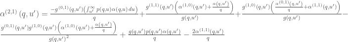
With $g\left(q,u\right) = \frac{1}{1 - P[q,\infty] - P[\infty,u] + P[q,u]}$

The procedure is to plug V.2) into V.1) and take 2 $q$ partial derivatives and 1 $u$ partial:

A. Inserting V.2) into V.1): $\alpha \left(q,u'\right)=\frac{\int_0^q g\left(q',u'\right) \int_{u'}^{\infty} \left(\int_{q'}^{\infty} p(q'',u) \alpha (q'',u) \, dq''\right) \, du \, dq'}{q}$
B. Take a $\frac{\partial}{\partial q}$ : $\alpha ^{(1,0)}\left(q,u'\right)=\frac{g\left(q,u'\right) \int_{u'}^{\infty} \left(\int_q^{\infty} p(q'',u) \alpha (q'',u) \, dq''\right) \, du}{q}-\frac{\int_0^q g\left(q',u'\right) \int_{u'}^{\infty} \left(\int_{q'}^{\infty} p(q'',u) \alpha (q'',u) \, dq''\right) \, du \, dq'}{q^2}$
C. Substitute A. into B. to eliminate integrals where applicable: $\alpha ^{(1,0)}\left(q,u'\right)=\frac{g\left(q,u'\right) \int_{u'}^{\infty} \left(\int_q^{\infty} p(q'',u) \alpha (q'',u) \, dq''\right) \, du}{q}-\frac{\alpha \left(q,u'\right)}{q}$
D. Take another $\frac{\partial}{\partial q}$ : $\alpha ^{(2,0)}\left(q,u'\right)=\frac{g^{(1,0)}\left(q,u'\right) \int_{u'}^{\infty} \left(\int_q^{\infty} p(q'',u) \alpha (q'',u) \, dq''\right) \, du}{q}-\frac{g\left(q,u'\right) \int_{u'}^{\infty} \left(\int_q^{\infty} p(q'',u) \alpha (q'',u) \, dq''\right) \, du}{q^2}-\frac{g\left(q,u'\right) \int_{u'}^{\infty} p(q,u) \alpha (q,u) \, du}{q}+\frac{\alpha \left(q,u'\right)}{q^2}-\frac{\alpha ^{(1,0)}\left(q,u'\right)}{q}$
E. Substitute C. into D to eliminate integrals where applicable: $\alpha ^{(2,0)}\left(q,u'\right)=\frac{g^{(1,0)}\left(q,u'\right) \left(\alpha ^{(1,0)}\left(q,u'\right)+\frac{\alpha \left(q,u'\right)}{q}\right)}{g\left(q,u'\right)}-\frac{g\left(q,u'\right) \int_{u'}^{\infty} p(q,u) \alpha (q,u) \, du}{q}-\frac{2 \alpha ^{(1,0)}\left(q,u'\right)}{q}$
F. Take a $\frac{\partial}{\partial u'}$ : $\alpha ^{(2,1)}\left(q,u'\right)=\frac{-g^{(0,1)}\left(q,u'\right) \left(\int_{u'}^{\infty} p(q,u) \alpha (q,u) \, du\right)}{q}+\frac{g^{(1,1)}\left(q,u'\right) \left(\alpha ^{(1,0)}\left(q,u'\right)+\frac{\alpha \left(q,u'\right)}{q}\right)}{g\left(q,u'\right)}+\frac{g^{(1,0)}\left(q,u'\right) \left(\frac{\alpha ^{(0,1)}\left(q,u'\right)}{q}+\alpha ^{(1,1)}\left(q,u'\right)\right)}{g\left(q,u'\right)}-\frac{g^{(0,1)}\left(q,u'\right) g^{(1,0)}\left(q,u'\right) \left(\alpha ^{(1,0)}\left(q,u'\right)+\frac{\alpha \left(q,u'\right)}{q}\right)}{g\left(q,u'\right)^2}+\frac{g\left(q,u'\right) p\left(q,u'\right) \alpha \left(q,u'\right)}{q}-\frac{2 \alpha ^{(1,1)}\left(q,u'\right)}{q}$
G. To get the result, substitute E. into F. to eliminate integrals where applicable.

[23] I could be wrong, and it’s hard to define what “reasonable” solutions look like. But I checked this three ways:

1. I tried numerically solving for $\alpha$ (and thus $\mathcal{I}$ ) assuming various joint probability distributions $p[q,u]$ — where $q$ and $u$ are dependent and generated by functions of Weibull, Pareto, Log-Normal, or Stable random variables. I didn’t see any solutions where $\alpha$ and $\mathcal{I}$ had significant $u$ -dependence without simultaneously having some other ridiculous feature (e.g. an infinity at small $q$ ).
2. I tried assuming $\alpha(q,u)$ had a few reasonable forms (e.g. $\alpha(q,u) \propto q^x u^{-y}$ ) and solving numerically for $p[q,u]$ . All the solutions I saw were not probability distributions (e.g. had negative probabilities).
3. It’s possible to solve the two integral equations directly if we assume that $p$ and $q$ are independent ( $p[q,u]=p_q[q]p_u[u]$ ) and the solutions are separable ( $\alpha(q,u)=\alpha_q(q)\alpha_u(u)$ and $\mathcal{I}(q,u)=\mathcal{I}_q(q)\mathcal{I}_u(u)$ ). In this case, $\mathcal{I}_q(q)$ and $\alpha_q(q)$ obey the same ODE as the original time-independent system in part I. And $\alpha_u(u)=\mathcal{I}_u(u)= constant$ , which isn’t realistic.

2 thoughts on “Price Impact in Efficient Markets”

Anonymous June 25, 2018 at 5:59 pm

very nice explaination

LikeLike

Reply ↓
Alain Rossier January 12, 2022 at 8:59 am

Thank you for this original way to look at the information-driven price impact.
How well do you think the assumptions I.1) and I.2) do in a market without colored prints, and with the presence of noise traders along with the informed trader executing a large metaorder?
Could you have similar arguments as in the Kyle’s model, where we supposed the existence of Bob, a market-maker that observes the meta-order (+ noise traders) and determines a clearing price so that Bob breaks even on average?

LikeLike

Reply ↓

Mechanical Markets

Price Impact in Efficient Markets

Definitions and Information-Driven Impact

I. A Bare-Bones Model

The integral denotes the quantity-averaged temporary impact “paid” over the course of an entire meta-order. “Fair pricing” means that, in aggregate, meta-orders of a given size do not earn excess returns or below-benchmark returns.

Relationship with Efficiency

Solving the System of Equations

Distribution of Order Sizes Implied by a Given Impact Curve

II. A Replacement Principle for Fair Pricing: Traders’ Effective Use of Price Targets

III. A Replacement Principle for Efficient Linkage, with Delayed Dissemination of Information

Where $q_d$ is a constant and $(q'-q_d)^+$ is the positive part of $(q'-q_d)$ : $max(0,(q'-q_d))$ .

IV. A Replacement Principle for Efficient Linkage, with Information Leakage from Sloppy Trading or Front-Running

V. Adding Time-Dependence

VI. A Weaker Constraint

Which says that, for a given $q$ , fair pricing holds on average across all $u$ .

Conclusion

2 thoughts on “Price Impact in Efficient Markets”

Leave a comment Cancel reply

Definitions and Information-Driven Impact

I. A Bare-Bones Model

The integral denotes the quantity-averaged temporary impact “paid” over the course of an entire meta-order. “Fair pricing” means that, in aggregate, meta-orders of a given size do not earn excess returns or below-benchmark returns.

Relationship with Efficiency

Solving the System of Equations

Distribution of Order Sizes Implied by a Given Impact Curve

II. A Replacement Principle for Fair Pricing: Traders’ Effective Use of Price Targets

III. A Replacement Principle for Efficient Linkage, with Delayed Dissemination of Information

Where is a constant and is the positive part of : .

IV. A Replacement Principle for Efficient Linkage, with Information Leakage from Sloppy Trading or Front-Running

V. Adding Time-Dependence

VI. A Weaker Constraint

Which says that, for a given , fair pricing holds on average across all .

Conclusion

Share this:

Related

2 thoughts on “Price Impact in Efficient Markets”

Leave a comment Cancel reply

Where $q_d$ is a constant and $(q'-q_d)^+$ is the positive part of $(q'-q_d)$ : $max(0,(q'-q_d))$ .

Which says that, for a given $q$ , fair pricing holds on average across all $u$ .